Conditional color formatting based on Rules
Prerequisite:
- Proceed with this page once you have mapped the Color/Legend fields with desired data fields for which you want conditional color formatting.
In case you want further information on prerequisite, click here.
Step 1
Select ‘Rules’ option from the dropdown menu of format style, then click ‘Add rule’ button to add rule(s) for formatting the colors in the visuals.
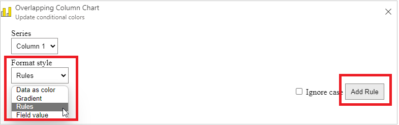
Go to Step 2 if you want to apply a color for the blank data values; otherwise, proceed to Step 3 (for numerical data values) or Step 4 (for text data values).
Step 2
a. Select ‘is Blank’ option from the drop-down menu and map desired color ( say ‘Pink’). It is used to apply a color for the empty data values in the Color field.
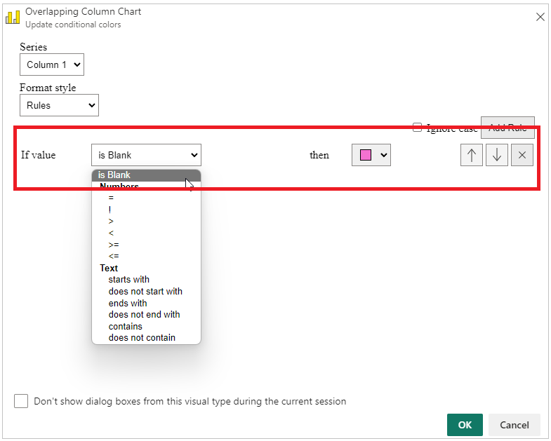
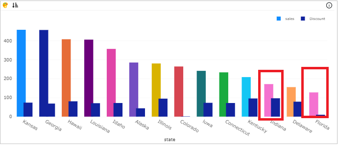
b. Click OK button to apply the rule. For example, ‘Indiana’ and ‘Florida’ have an empty value in the color field, so these bars have changed to 'Pink' color. The selected Power BI theme colors applied by default to the remaining data values as shown below:
Step 3
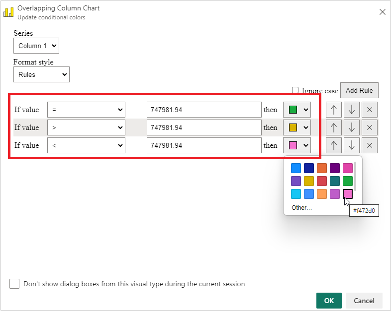
a. Select any one comparison symbol and enter the value that you want to compare with all the data values in the color field, then select the desired color from the color palette.
For example, map ‘Brand name’, ‘Current Sales’, and ‘Previous Sales’ to ‘X-axis’ (category), ‘Y-axis-1’ and ‘Y-axis-2’ respectively. Map ‘Current Sales’ to Color 1 field in the visualization pane. The data table and field mapping as follows:
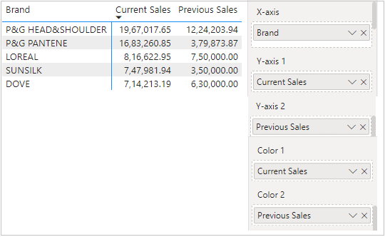
b. Select any current sales value from the table that you wish to apply the color in the visual (say 7,47,981.94). Select ‘Green’ color if sale is equal to 7,47,981.94, Select ‘Yellow’ color if sale is greater than 7,47,981.94, and select ‘Pink’ color if sale is lesser than 7,47,981.94 as below:
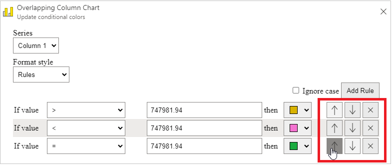
c. Place the rules in the desired order by clicking the "Arrow up" and "Arrow down" buttons. Click ‘X’ button to remove the rule from the list.
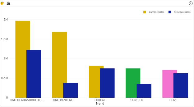
d. Click OK button to apply the conditional colors. The Brand 'SUNSILK' is highlighted with ‘Green’ color as its ‘Current Sales’ value is equal to 7,47,981.94. Similarly, ‘P&G HEAD&SHOULDER’, ‘P&G PANTEE’ and ‘LOREAL’ brands have ‘Current Sales’ more than 7,47,981.94.
Step 4
a. Map Color 2 field with text-based values (say ‘Brand’), then select ‘Column 2’ from the Series drop-down. Select suitable rule(s) as per your requirements:
- Starts with
- Does not starts with
- Ends with
- Does not ends with
- Contains
- Does not contain
A mapped color could be applied to that specific data value if the input text satisfied the selected rule.
- Note: To disable case-sensitivity for input text, use the Ignore case checkbox.
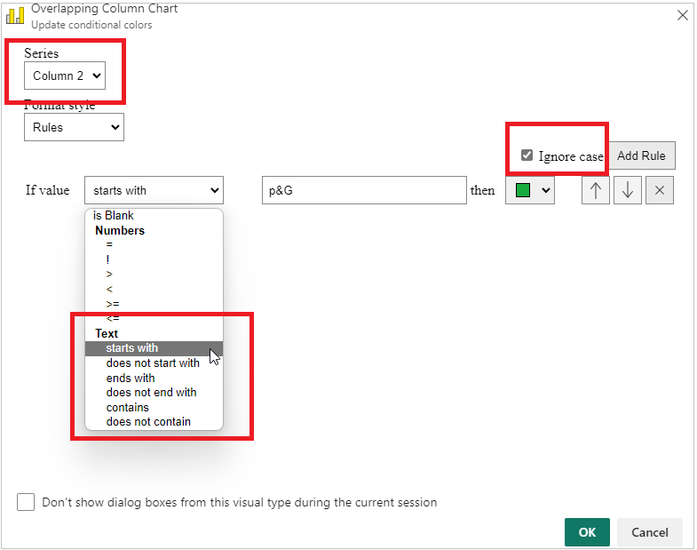
b. For example, in the first rule, Select ‘Starts with’ rule and enter the input text ‘p&G’ and map ‘Green’ color to it.
For the second rule: Select ‘Contains’ rule and enter the input text ‘Un’ and map ‘Yellow’ color to it.
For the third rule: Select ‘Ends with’ rule and enter the input text ‘ve’ and map ‘Pink’ color to it.
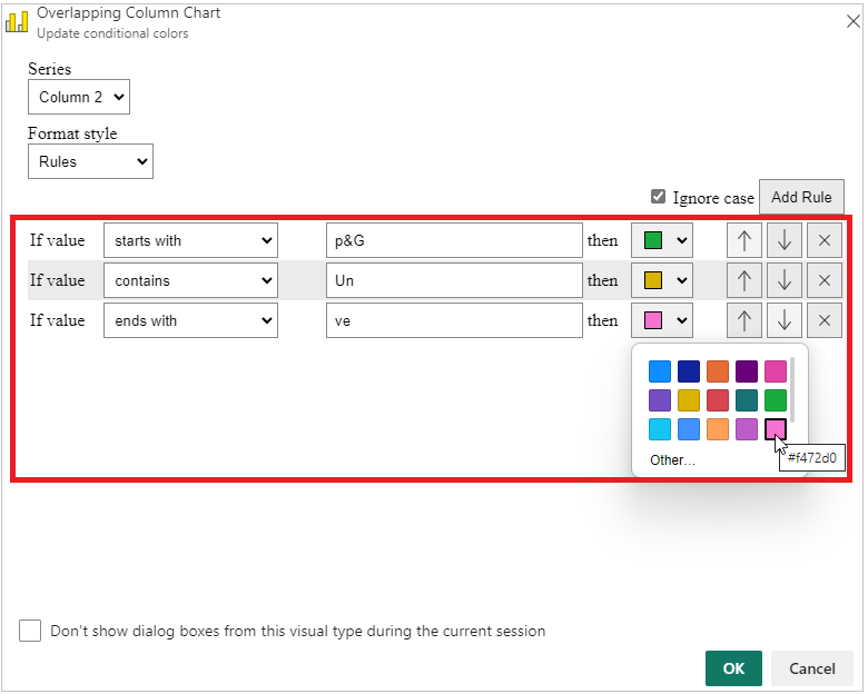
c. Click OK button to apply the mentioned rules to the visual.
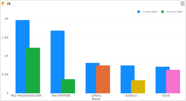
Note: The rules are executed in the same sequence as you specified in the dialog box.